Before you begin
Resource allocation and competing uses →The question
What changes when a continuous plan must make discrete decisions?
Learning objectives
- 01Recognize sets, parameters, variables, objectives and constraints in a deployment model.
- 02Explain when integer variables are needed.
- 03Interpret feasibility, shadow values and scenario comparison without equating optimality with truth.
Core explanation
A linear program represents continuous decisions with linear objectives and constraints. In a supply system, variables might be tonnes shipped from source to facility, production by technology and unmet demand. Constraints enforce supply, capacity, balances and demand; the objective may minimize cost or emissions. Linearity supports transparent and scalable analysis when relationships are appropriate.
Mixed-integer programming adds discrete choices: whether to build a facility, select a technology, open a depot or use a transport mode. Binary decisions can represent fixed costs and logical conditions but make models harder to solve. Piecewise linear approximations can represent selected nonlinear behavior, provided approximation error is reported.
An optimum is conditional on data, structure and objective. Check units, conservation, infeasibility, unused capacity, binding constraints, alternative near-optimal solutions and sensitivity. Pyomo provides a transparent modeling environment, but a solver certificate does not validate the scientific assumptions.
Key concepts
Decision variable
A quantity selected by the model within defined bounds and logic.
Constraint
A mathematical condition representing a physical, policy, contractual or logical limit.
Binary variable
A zero-or-one decision used for choices such as building or not building.
Binding constraint
A limit reached at the solution that can explain scarcity or trade-offs.
Visual explanation
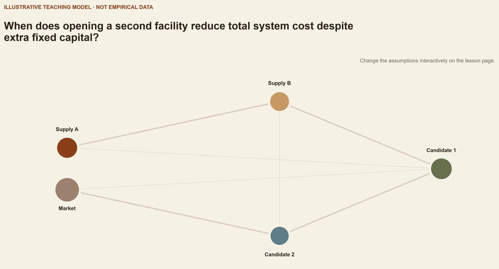
Explore · mini lp milp solver
Distinguish continuous flows from binary facility and technology choices.
Allocate six supply units, then switch one candidate facility on or off and inspect feasibility.
iIllustrative learning model — values are not scientific results or forecasts.
Remaining
Plant A · open
0/4Plant B · binary choice
0/4Carry inventory
0/2Allocate six supply units, then switch one candidate facility on or off and inspect feasibility.
Worked example
A two-source, two-facility LP
Allocate two feedstocks to two candidate facilities while meeting demand and respecting supply and capacity.
- 01
Define shipment variables and a total delivered-cost objective.
- 02
Add source supply, facility capacity, quality and demand constraints.
- 03
Compare the optimum with a resilient near-optimal solution that diversifies supply.
A small cost difference may buy substantial resilience; alternative optima are decision information.
Case file
Pyomo: modeling and solving mathematical programs in Python
- Why it is here
- Pyomo illustrates an auditable algebraic modelling workflow.
- What to inspect
- Inspect how model components stay separate from solver choice.
- Limitation
- A modelling language does not validate data, objectives or stakeholder legitimacy.
Tool in context
Pyomo
- Use it for this task
- Express variables, constraints and objectives transparently in an optimization model.
- Limitation
- A mathematically optimal result inherits every omission and bias in the model and data.
Inputs, outputs & scope
- What it is
- An open-source Python environment for formulating and analysing optimization models.
- Problem it addresses
- How can decisions, objectives and constraints be represented transparently?
- Inputs
- Sets, parameters, variables, objectives, constraints and a compatible solver.
- Outputs
- Feasible or optimized decisions, objective values and diagnostic information.
- Typical applications
- LP/MILP allocation, siting, supply chains, scenarios and multi-objective analysis.
Core references
- Hart, Watson and Woodruff (2011). Pyomo: modeling and solving mathematical programs in Python.https://doi.org/10.1007/s12532-011-0026-8 ↗
- Hamid Ghaderi, Mir Saman Pishvaee and Alireza Moini (2017). Biomass supply chain network design: An optimization-oriented review and analysis.https://doi.org/10.1016/j.indcrop.2016.09.027 ↗
Further reading +1
- Pyomo project (2026). Pyomo optimization modeling documentation.Open source ↗
Knowledge check
Key takeaway
LP/MILP makes deployment logic auditable; it does not make incomplete priorities or data objective.
A solver’s optimal status proves that the recommended plan is complete, fair and deployable.
Units and balances, source of every parameter, omitted constraints, alternative solutions, infeasibility diagnostics and sensitivity.